Efficient and principled score estimation

New paper online: Score matching goes Nystrom. With guarantees!

We propose a fast method with statistical guarantees for learning an exponential family density model where the natural parameter is in a reproducing kernel Hilbert space, and may be infinite dimensional. The model is learned by fitting the derivative of the log density, the score, thus avoiding the need to compute a normalization constant. We improved the computational efficiency of an earlier solution with a low-rank, Nystr\”om-like solution. The new solution retains the consistency and convergence rates of the full-rank solution (exactly in Fisher distance, and nearly in other distances), with guarantees on the degree of cost and storage reduction. We evaluate the method in experiments on density estimation and in the construction of an adaptive Hamiltonian Monte Carlo sampler. Compared to an existing score learning approach using a denoising autoencoder, our estimator is empirically more data-efficient when estimating the score, runs faster, and has fewer parameters (which can be tuned in a principled and interpretable way), in addition to providing statistical guarantees.

https://arxiv.org/abs/1705.08360

Google Summer of Code 2016

Great news: Shogun just got accepted to the GSoC 2016. After our break year in 2015, we are extremely excited to continue our GSoC tradition starting in 2011 (when I first joined Shogun).

If you are a student and wish to spend the summer hacking Machine Learning, guided by a vibrant international community of academics, professionals, and NERDS, then pay us a visit. Oh, and you will receive a cheque over $5000 from Google.

This year, we focus on framework improvements rather than solely adding new algorithms. Consequently, most projects have a heavy focus on packaging and software engineering questions. But there will be Machine Learning too. We are aiming high!

Check our our ideas list and read how to get involved.

Kamiltonian Monte Carlo

Together with Dino, Sam, Zoltan, and Arthur, I recently arxived a first draft published an article on a project that combines two topics — the combination of which I find rather exciting: kernel methods and Hamiltonian Monte Carlo.

Updates.

Here is the abstract.

We propose Kamiltonian Kernel Hamiltonian Monte Carlo (KMC), a gradient-free adaptive MCMC algorithm based on Hamiltonian Monte Carlo (HMC). On target densities where classical HMC is not an option due to intractable gradients, KMC adaptively learns the target’s gradient structure by fitting an exponential family model in a Reproducing Kernel Hilbert Space. Computational costs are reduced by two novel efficient approximations to this gradient. While being asymptotically exact, KMC mimics HMC in terms of sampling efficiency, and offers substantial mixing improvements over state-of-the-art gradient free samplers. We support our claims with experimental studies on both toy and real-world applications, including Approximate Bayesian Computation and exact-approximate MCMC.

Motivation: HMC with intractable gradients.

Many recent applications of MCMC focus on models where the target density function is intractable. A very simple example is the context of Pseudo-Marginal MCMC (PM-MCMC), for example in Maurizio’s paper on Bayesian Gaussian Processes classification. In such (simple) models the marginal likelihood $p(\mathbf{y}|\theta )$ is unavailable in closed form, but only can be estimated. Performing Metropolis-Hastings style MCMC on $\hat{p}(\theta |\mathbf{y})$ results in a Markov chain that (remarkably) converges to the true posterior. So far so good. But no gradients.

Sometimes, people argue that for simple objects as latent Gaussian models, it is possible to side-step the intractable gradients by running an MCMC chain on the joint space $(\mathbf{f},\theta)$ of latent variables and hyper-parameters, which makes gradients available (and also comes with a set of other problems such as high correlations between $\mathbf{f}$ and $\theta$,  etc). While I don’t want to get into this here (we doubt existence of a one-fits-all solution), there is yet another case where gradients are unavailable.

Approximate Bayesian Computation is based on the context where the likelihood itself is a black-box, i.e. it can only be simulated from. Imagine a physicist coming to you with three decades of intuition in the form of some Fortran code, which contains bits implemented by people who are not alive anymore — and he wants to do Bayesian inference on the code-parameters via MCMC… Here we have to give up on getting the exact answer, but rather simulate from a biased posterior. And of course, no gradients, no joint distribution.

proposals_FlowerState-of-the-art methods on such targets are based on adaptive random walks, as no gradient information is available per-se. The Kameleon (KAMH) improves over other adaptive MCMC methods by constructing locally aligned proposal covariances. Wouldn’t it be cooler to harness the power of HMC?

Kamiltonian Monte Carlo starts as a Random Walk Metropolis (RWM) and then smoothly transitions into HMC. It explores the target at least as fast as RWM (we proof that), but improves the mixing in areas where it has been before.

We do this by learning the target gradient structure from the MCMC trajectory in an adaptive MCMC framework — using kernels. Every MCMC iteration, we update our gradient estimator with a decaying probability $a_t$ that ensures that we never stop updating, but update less and less, i.e. $$\sum_{t=1}^\infty \frac{1}{a_t}=\infty\qquad\text{and}\qquad\sum_{t=1} ^\infty \frac{1}{a_t^2}=0.$$ Christian Robert challenged our approach: using non-parametric density estimates for MCMC proposals directly is a bad idea: if certain parts of the space are not explored before adaptation effectively stopped, the sampler will almost never move there. For KMC (and for KAMH too) however, this is not a problem: rather than using density estimators as proposal directly, we use them for proposal construction. This way, these algorithms inherit ergodicity properties from random walks. I coded an example-demo here.

Kernel exponential families as gradient surrogates.
The density (gradient) estimator itself is an infinite dimensional exponential family model. More precisely, we model the un-normalised target log-density $\pi$ as an RKHS function $f\in\mathcal{H}$, i.e. $$\text{const}\times\pi(x)\approx\exp\left(\langle f,k(x,\cdot)\rangle_{{\cal H}}-A(f)\right),$$ which in particular implies $\nabla f\approx\nabla\log\pi.$ Surprisingly, and despite a complicated normaliser $A(f)$, such a model can be consistently fitted by directly minimising the expected $L^2$ distance of model and true gradient, $$J(f)=\frac{1}{2}\int\pi(x)\left\Vert \nabla f(x)-\nabla\log \pi (x)\right\Vert _{2}^{2}dx.$$ The magic word here is score-matching. You could ask: “Why not use kernel density estimation?” The answer: “Because it breaks in more than a few dimensions.” In contrast, we are actually able to make the above gradient estimator work in ~100 dimensions on Laptops.

Two approximations.
The über-cool infinite exponential family estimator, like all kernel methods, doesn’t scale nicely in the number $n$ of data used for estimation — and here neither in the in input space dimension $d$. Matrix inversion with costs $\mathcal{O}(t^3d^3)$ becomes a blocker, in particular as $t$ here is the growing number of MCMC iterations. KMC comes in two variants, which correspond to different approximations to the original kernel exponential family model.

  1. KMC lite expresses the log-density in a smaller dimensional (yet growing) sub-space, via collapsing all $d$ input space dimensions into one. It takes the dual form $$f(x)=\sum_{i=1}^{n}\alpha_{i}k(x_{i},x),$$ where the $x_i$ are $n$ random sub-samples (just like KAMH) from the Markov chain history. Downside: KMC lite has to be re-estimated whenever the $x_i$ change. Advantage: The estimator’s tails vanish outside the $x_i$, i.e. $\lim_{\|x\|_{2}\to\infty}\|\nabla f(x)\|_{2}=0$, which translates into a geometric ergodicity result as we will see later.
  2. KMC finite approximates the model as a finite dimensional exponential family in primal form, $$f(x)=\langle\theta,\phi_{x}\rangle_{{\cal H}_{m}}=\theta^{\top}\phi_{x},$$ where $x\in\mathbb{R}^{d}$ is embedded into a finite dimensional feature space $\phi_{x}\in{\cal H}_{m}=\mathbb{R}^{m}.$ While other choices are possible, we use the Randon Kitchen Sink framework: a $m$-dimensional data independent random Fourier basis. Advantage: KMC lite is an efficient on-line estimator that can be updated at constant costs in $t$ — we can fit it on all of the MCMC trajectory. Disadvantage: Its do not decay and our proof for geometric ergodicity of KMC lite does not apply.

KMC

Increasing dimensions.
So far, we did not work out how the approximation errors propagate through the kernel exponential family estimator, but we plan to do that at some point. The paper contains an empirical study which shows that the gradients are good enough for HMC up to ~100 dimensions — Under a “Gaussian like smoothness” assumption. The below plots show the acceptance probability along KMC trajectories and quantify how “close” KMC proposals are to HMC proposals.

From RWM to HMC.
Using the well known and (ab)used Banana density as a target, we feed a non-adaptive version of KMC and friends with an increasing number of so-called “oracle” samples (iid from the target), and then quantify how well they mix. While this scenario is totally straw-man, it allows to compare the mixing behaviour of the algorithms after a long burn-in. The below plots show KMC transitioning from a random walk into something close to HMC as the number of “oracle” samples (x-axis) increases.kmc_banana_mixingABC — Reduced simulations and no additional bias.
While there is another example in the paper, I want to show the ABC one here, which I find most interesting. Recall in ABC, the likelihood is not available. People often use synthetic likelihoods that are for example Gaussian, which induces an additional bias (in addition to ABC itself) but might improve statistical efficiency. In an algorithm called Hamiltonian ABC, such a synthetic likelihood is combined with stochastic gradient HMC (SG-HMC)  via randomized finite differences, called simultaneous perturbation stochastic approximation (SPSA), which works as follows. To evaluate the gradient at a position $\theta$ in sampling space:

  1. Generate a random SPSA mask $\Delta$ (set of binary directions) and compute the perturbed $\theta+\Delta$ and $\theta+\Delta$.
  2. Interpolate linearly between them the perturbations. That is simulate from the ABC likelihood at both points, construct the synthetic likelihood, and use their difference.
  3. The gradient is a (step-size dependent!) approximation to the unknown gradient of the (biased) synthetic likelihood model.
  4. Perform a single stochastic HMC leapfrog step (adding friction as described in the SG-HMC paper)
  5. Iterate for $L$ leapfrog iterations.

What I find slightly irritating is that this algorithm needs to simulate from the ABC likelihood in every leapfrog iteration — and then discards the gained information after a leapfrog step has been taken. How many leapfrog steps are common in HMC? Radford Neal suggests to start with  $L\in[100,1000]$. Quite a few ABC simulations come with this! But there are more issues:

  1. SG-HMC mixing. I found that stochastic gradient HMC mixes very poorly when the gradient noise large. Reducing noise costs even more ABC simulations. Wrongly estimated noise (non-stationary !?!) induces bias due to the “always accept” mentality. Step-size decreasing to account for that further hurts mixing.
  2. Bias. The synthetic likelihood can fail spectacularly, if the true likelihood is skewed for example.

KMC does not suffer from either of those problems: It keeps on improving its mixing as it sees more samples, while only requiring a single ABC simulation at each MCMC iterations — rather than HABC’s $2L$ (times noise-reduction-repetitions). It targets the true (modulo ABC bias) posterior, while accumulating information of the target (and its gradients) in the form of the MCMC trajectory.

On a Log-Gaussian likelihood

But how do you choose the kernel parameter?
Often, this question is a threat for any kernel-based algorithm. For example, for the KAMH algorithm, it is completely unclear (to us!) how select these parameters in a principled way. For KMC, however, we can simply use cross-validation on the score matching objective function above. In practice, we use a black box optimisation procedure (for example CMA or Bayesian optimisation) to on-line update the kernel hyper-parameters every few MCMC iterations. See an example where our Python code does this here. Just like the updates to the gradient estimator itself, this can be done with a decaying probability to ensure asymptotic correctness.

Unbiased Big Bayes without sub-sampling bias: Paths of Partial Posteriors

Together with Dino Sejdinovic and Mark Girolami, I recently arxived our second draft of a paper on the popular topic of how to scaleup Bayesian inference when facing large datasets.

This project is yet another method to scale up Bayesian inference via sub-sampling. But unlike most other work on this field, we do not use sub-sampling within an MCMC algorithm to simulate from the posterior distribution of interest. Rather, we use sub-sampling to create a series of easier inference problems, whose results we then combine to get the answer to the question we were originally asking — in an estimation sense, without full posterior simulation. I’ll describe the high-level ideas now.

Updates on the project:

Let’s assume the following desiderata for large-scale Bayesian estimators:

  • Average computational costs sub-linear in the data size $N$.
  • Bounded variance (even for growing $N$) and can be controlled.
  • No sub-sampling bias is introduced. The method inherits the usual finite time bias from MCMC though.
  • Not limited to certain models or inference schemes.
  • Trade off redundancy in the data against computational savings.
  • Perform competitive in practice.

Bayesian inference usually involves integrating a functional $\varphi:\Theta\rightarrow\mathbb{R}$ over a posterior distribution $$\phi=\int d\theta\varphi(\theta)\underbrace{p(\theta|{\cal D})}_{\text{posterior}},$$ where $$p(\theta|{\cal D})\propto\underbrace{p({\cal D}|\theta)}_{\text{likelihood data}}\underbrace{p(\theta)}_{\text{prior}}.$$ For example, to compute the predictive posterior mean for a linear regression model. This is often done by constructing an MCMC algorithm to simulate $m$ approximately iid samples from approximately $\theta^{(j)}\sim p(\theta|{\cal D})$ (the second “approximately” here refers to the fact that MCMC is biased for any finite length of the chain, and the same is true for our method) and then performing Monte Carlo integration $$\phi\approx\frac{1}{m}\sum_{j=1}^{m}\varphi(\theta^{(j)}).$$ Constructing such Markov chains can quickly become infeasible as usually, all data needs to be touched in every iteration. Take for example the standard Metropolis-Hastings transition kernel to simulate from $\pi(\theta)\propto p(\theta|{\cal D})$, where at a current point $\theta^{(j)}$, a proposed new point $\theta’\sim q(\theta|\theta^{(j)})$ is accepted with probability $$\min\left(\frac{\pi(\theta’)}{\pi(\theta^{(j)})}\times\frac{q(\theta^{(j)}|\theta’)}{q(\theta’|\theta^{(j)})},1\right).$$ Evaluating $\pi$ requires to iterate through the whole dataset. A natural question therefore is: is it possible to only use subsets of $\mathcal{D}$?

Existing work. There has been a number of papers that tried to use sub-sampling within the transition kernel of MCMC:

All these methods have in common that they either introduce bias (in addition to the bias caused by MCMC), have no convergence guarantees, or mix badly. This comes from the fact that it is extremely difficult to modify the Markov transition kernel and maintain its asymptotic correctness.

In our paper, we therefore take a different perspective. If the goal is to solve an estimation problem as the one above, we should not make our life hard trying to simulate. We construct a method that directly estimates posterior expectations — without simulating from the full posterior, and without introducing sub-sampling bias.

The idea is very simple:

  1. Construct a series of partial posterior distributions $\tilde{\pi}_{l}:=p({\theta|\cal D}_{l})\propto p({\cal D}_{l}|\theta)p(\theta)$ from subsets of sizes $$\vert\mathcal{D}_1\vert=a,\vert\mathcal{D}_2\vert=2^{1}a,\vert\mathcal{D}_3\vert=2^{2}a,\dots,\vert\mathcal{D}_L\vert=2^{L-1}a$$ of the data. This gives $$p(\theta)=\tilde{\pi}_{0}\rightarrow\tilde{\pi}_{1}\rightarrow\tilde{\pi}_{2}\rightarrow\dots\rightarrow\tilde{\pi}_{L}=\pi_{N}=p({\theta|\cal D}).$$
  2. Compute posterior expectations $\phi_{t}:=\hat{\mathbb{E}}_{\tilde{\pi}_{t}}\{\varphi(\theta)\}$ for each of the partial posteriors. This can be done for example MCMC, or other inference methods. This gives a sequence of real valued partial posterior expectations — that converges to the true posterior.
  3. Use the debiasing framework, by Glynn & Rhee. This is a way to unbiasedly estimate the limit of a sequence without evaluating all elements. Instead, one randomly truncates the sequence at term $T$ (which should be “early” in some sense, $T$ is a random variable), and then computes $$\phi^*=\sum_{t=1}^T \frac{\phi_{t}-\phi_{t-1}}{\mathbb{P}\left[T\geq t\right]}.$$ This is now an unbiased estimator for the full posterior expectation. The intuition is that one can rewrite any sequence limit as a telescopic sum $$\lim_{t\to\infty} \phi_t=\sum_{t=1}^\infty (\phi_{t}-\phi_{t-1})$$ and then randomly truncate the infinite sum and divide through truncation probabilities to leave the expectation untouched, i.e. $$\mathbb{E}[\phi^*]=\phi,$$where $\phi$ is the sequence limit.
  4. Repeat $R$ times for reducing the estimator variance as $1/R$.

In the paper, we choose the random truncation time as $$\mathbb{P}(T=t)\propto 2^{-\alpha t}.$$ From here, given a certain choice of $\alpha$, it is straight-forward to show the average computational cost of this estimator is $\mathcal{O} (N^{1-\alpha}),$ which is sub-linear in $N$. We also show that variance is finite and can be bounded even when $N\to\infty$. This statement is modulo certain conditions on the $\phi_t$. In addition, the choice of the $\alpha$-parameter of the random truncation time $T$ is crucial for performance. See the paper for details how to set it.

Experimental results are very encouraging. On certain models, we are able to estimate model parameters accurately before plain MCMC even has finished a single iteration. Take for example a log-normal model $$p(\mu,\sigma|{\cal D})\propto\prod_{i=1}^{N}\log{\cal N}(x_{i}|\mu,\sigma^{2})\times\text{flat prior}$$ and functional $$\varphi((\mu,\sigma))=\sigma.$$ We chose the true parameter $\sigma=\sqrt{2}$ and ran our method in $N=2^{26}$ data. The pictures below contain some more details.

Comparison to stochastic variational inference is something we only thought of quite late in the project. As we state in the paper, as mentioned in my talks, and as pointed out in feedback from the community, we cannot do uniformly better than MCMC. Therefore, comparing to full MCMC is tricky — even though there exist trade-offs of data redundancy and model complexity that we can exploit as showed in the above example. Comparing to other “limited data” schemes really showcases the strength (and generality) of our method.

We chose to compare against “Gaussian Processes for Big Data“, which puts together a decade of engineering of variational lower bounds, the inducing features framework for GPs, and stochastic variational inference to solve Gaussian Process regression on roughly a million data points. In contrast, our scheme is very general and not specifically designed for GPs. However, we are able to perform similar to this state of the art method. On predicting airtime delays, we reach a slightly lower RMSE at comparable computing effort. The paper contains details on our GP, which is slightly different (but comparable) to the one used in the GP for Big Data paper. Another neat detail of the GP example is that the likelihood does not factorise, which is in contrast to most other Bayesian sub-sampling schemes.

In summary, we arrive at

  • Computational costs sub-linear in $N$
  • No introduced sub-sampling bias (in addition to MCMC, if used)
  • Finite, and controllable variance
  • A general scheme that is not limited to MCMC nor to factorising likelihoods
  • A scheme that trades off redundancy for computational savings
  • A practical scheme that performs competitive to state-of-the-art methods and that has no problems with transition kernel design.
  • See the paper for a list of weaknesses and open problems.

Shogun 4.0 and GSoC 2014 follow up

No, this is not about Fernando’s and mine honeymoon …

The Shogun team just released version 4.0 of their community driven Machine Learning toolbox. This release most of all features the work of our 8 Google Summer of Code 2014 students, so this blog post is dedicated to them — you guys rock. This also brings an end to yet another very active year of Shogun: we organised a second workshop in Berlin, and I presented Shogun in to the public in London, New York and Berlin.

For the 4th time, Shogun participated in Google’s wonderful program which more than anything boosted the team’s size and motivation. What else makes people spend sleepless nights hunting bugs for the sake of Machine Learning for everyone? This year was the first time that I organised our participation. This ranged from writing the application last second, harrassing potential mentors until they say ‘yes’, to making up overly ambitious projects to scare students away, and ending up mentoring too many students on my own. Jokes aside, this was a very challenging (in particular time-wise) but also a very rewarding experience that definitely sharpened my project organisation skills. As in the previous year, I tried to fuse my scientific life and Shogun’s GSoC participation — kernel methods and variational learning is something I touch on a daily basis at Gatsby. Many mentors were approached after having met them at scientific Machine Learning conferences, and being exposed to ML on for some years now, it is also easier to help students implement and write about popular ML algorithms.
Here is a list. (Note that all projects come with really nice IPython notebooks — something that we continued to insist on from last year.)

Fundamental ML algorithms by Parijat Mazumdar (parijat). Mentor: Fernando
Shogun needs more standard ML algorithms. Parijat implemented some of those: random forests, kernel density estimation and more. Parijat’s code quality is amazing and together with Fernando’s superb mentoring skills (his first time mentoring), this project is likely to have been very sustainable.
Notebook random forest, notebook KDE.

Kernel testing and feature selection by Rahul De (lambday). Mentor: Dino Sejdinovic, Heiko
Previous year’s student lambday continued to rock. First, he massively extended my 2012 project on kernel hypothesis testing to Big Data land. Dino, who was one of the invited speakers in the Shogun workshop last summer, and I are actually working on a journal article where we will use this code. Second, he extended the framework to perform feature selection via dependence measures. Third, he initiated and guided development of a framework for unifying Shogun’s linear algebra operations. This for example can be used to change existing algorithms from CPU to GPU with a compile switch — useful also for our deep learning project.

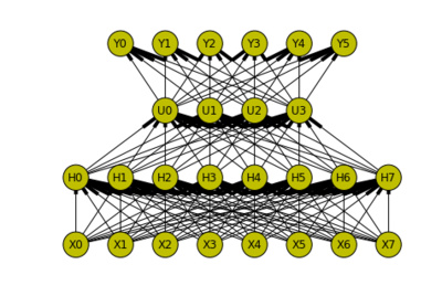
Variational Inference for Gaussian Processes by Wu Lin (yorkerlin). Mentor:Heiko, Emtiyaz Khan
In our third GSoC project on GPs, Wu took a couple of state-of-the-art approximate variational inference methods developed by Emiyaz, and put them into Shogun’s framework. The result of this very involved and technical project is that we now have large-scale classification using GPs. Emtiyaz also was a speaker at ourworkshop.
Notebook

Shogun missionary by Saurabh. Mentor:Heiko
The idea of this project was to showcase Shogun’s abilities — sometimes we definitely need to work on. Saurabh wrote a couple of Notebooks that are essentially ML tutorials using Shogun. If you want to know about ML basics, regression, classification, model-selection, SVMs, multiclass, multiple kernel learning this was for you. He also extended our web-demo framework to for example include model-selection for GPs.

OpenCV integration by Kislay. Mentor: Kevin
Kislay, after writing a very cool notebook on PCA for his application, wrote data-structures to bridge between Shogun and OpenCV. The project was supervised by Kevin, who is also one of our former GSoC students This makes it possible to use the too libraries together in a neat way.

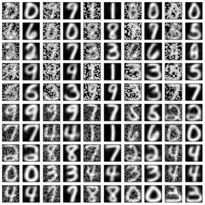
Deep learning by Khaled Nasr. Mentor: Theofanis, Sergey
The hype is on! After NIPS, Facebook, GoogleDeepmind, Shogun now also joined 😉 Khaled did a very good job in coding up the standard ones, and was involved in generalising Shogun’s linear algebra on the fly with lambday. This is a project that is likely to have a second part. Check his superb notebooks on deep belief neural networks, convolutional networks,autoencoders, restricted Boltzman machines

SO Learning with Approximate Inference by Jiaolong. Mentor: hushell, Thoralf

This was another project that was (co-)mentored by a former GSoC student. With the help his mentors, Jialong implemented various approximate inference methods for structured output (SO) models. Check out his notebook.


Large-Scale Multi-Label Classification by Abinash. Mentor: Thoralf
Another project involving our structured output expert Thoralf as mentor. Abinash implemented large-scale multilabel learning — beating scikit learn‘s implementation both in runtime and accuracy. The last experiment is described in this notebook.

Finally, we sent two of our delegates (Thoralf and Fernando) to the 10th year jubilee mentor summit in California in late October. Really cool: I got lucky and won Google’s lottery on some extra places, so I could also join. The summit once again was overly colourful, bursting with creative minds who have the most diverse set of opinions and approaches, but who are all united by their excitement about open-source. The beauty of this community to me really lies in the people who do work purely driven by their interest on *the thing itself*, independent of competitive and in particular commercial interests — sometimes almost to an extend that is beyond any form of compromise. A wonderful illustration of this was when at the mentor summit, during the reception in the Tech museum in San Jose: Google’s speaker and head of finance Patrick Pichette (disclaimer: not sure, don’t quote me on this) who is the boss of Chris DiBona, who himself organises the GSoC, searched to inspire the audience to “think BIG” and to “change the lifes of GSoC students”. Guest speaker Linus Torvalds 10 minutes later then contemplates that he could not be a GSoC mentor as he would scare people away and that the best way to get involved in open-source is to “start small” — a sentence after which P.P. left the room. Funny enough: in GSoC, this community is then hugged by a super capitalistic American internet company — and gladly lets it happen: we all love GSoC and Shogun certainly would not be where it is without it. I also want to mention the day Google rented a whole theme park for us nerds — which made Fernando try a roller-coaster for the first time after being pushed by MLPack maintainer Ryan and myself. After being horrified at first, he even started to talk about C++ the second or third time.

As you would expect from attending such geeky meetings, Thoralf, Fernado, and I also spent quite some time hacking Shogun, discussing ideas until late night (of course getting emotional about them 🙂 ). I managed to take a picture of Fernando falling asleep while hacking Shogun’s modular interfaces. Some of those ideas are collected on our wiki.

  • Improve usability
  • Making Shoun more modular and slim
  • Improving Shogun’s efficiency

Some of those ideas are also part of our theme for our GSoC 2015 application and our planned Hackathon. We have come to a point where we seriously need to focus on application and stability rather than adding more and more cutting-edge algorithms — Shogun’s almost 15 year old framework needs a face lift. GSoC students will see that this years project ideas will focus on cleaning up the toolbox and implement ML applications.

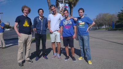
Meet the Shogun/MLPack crew, as nerdy as it gets 😉

Shogun in NYC

In late August, I was invited to NYC to present Shogun at an open-source Machine Learning software workshop (link), organised by John Langford. Seeing Shogun being recognised as a major player along with big ML/stats libraries like TheanoStanTorchLibLinearVowpalWabbit, etc really got my excited.

I talked to most of the other project’s developers and a few very interesting possible collaborations came up. For example, Shogun’s unique way to automagically generate interfaces to most computing languages via swig. It has been in our pipeline of ideas for a long time to pull this functionality out of Shogun, and offer it to other projects in a modular way. Sergey has put together (link) a simple prototype here and will continue to work on this soon.

Another thing is that we would like to integrate some (fixed) models from Stan into Shogun, for example to complement our collection of variational inference methods for Gaussian Processes with a full blown MCMC based approach.

While talking to Gunnar Raetsch, we had the idea to host a hackfest where we bring together all Shogun core-developers for a week, working on more sophisticated projects that are not suitable for Google Summer of Code. A generic framework for parallelising/distributing algorithms in Shogun would be a first idea, extending ideas from lambday’s GSoC 2013 project. This would again also be useful for other ML libraries and I in fact talked to John Langford about using ideas from VowpalWabbit here. We made a list of ideas (link) for such a hack and are currently trying to get funding for it.

The meeting was video-taped and I will put links for this soon.

Shogun workshop 2014

Another super nice event that happened in Berlin in July was the second Shogun workshop that me and the Shogun team organised. We had a hands-on session and a main workshop day full of talks, cool people, and lots of Machine Learning. It is a great pleasure working with the Shogun team, and I am very happy that we were able to push this year’s workshop through.

I talked a bit about what Shogun is and what it tries to be, and gave some directions for future work. If you missed the event, we got full video coverage!

Workshop program

Videos

Shogun at EuroPython 2014

It’s already a while ago, in July, I presented Shogun at the EuroPython in Berlin. This was a super nice conference full of interesting people and projects. My talk was recorded and can be found [here], slides are [here].

Another super interesting project was presented by Thomas Wiecki: Probabilistic programming with PyMC3 [video]. This is a very interesting project, a bit similar to Stan, which allows to plug together probabilistic models and then do HMC for inference, powered by automatic differentiation (which I am currently super excited about). Unlike Stan, this happens all in Python which makes things super comfortable (example notebook). As I am working on kernel-based samplers (Kameleon MCMC & soon more), this might be a good vehicle to make them public, exploiting the nice auto-diff tool (Theano) that PyMC uses.

ICML paper: Kernel Adaptive Metropolis Hastings

$\DeclareMathOperator*{\argmin}{arg\,min}$ $\def\Mz{M_{\mathbf{z},y}}$

In this year’s ICML in Bejing, Arthur Gretton, presented our paper on Kernel Adaptive Metropolis Hastings [link, poster]. His talk slides are based on Dino Sejdinovic ones [link]. Pitty that I did not have travel funding. The Kameleon is furious!

The idea of the paper is quite neat: It is basically doing Kernel-PCA to adapt a random walk Metropolis-Hastings sampler’s proposal based on the Markov chain’s history. Or, more fancy: Performing a random walk on an empirically learned non-linear manifold induced by an empirical Gaussian measure in a Reproducing Kernel Hilbert Space (RKHS). Sounds scary, but it’s not: the proposal distribution ends up being a Gaussian aligned to the history of the Markov chain.

We consider the problem of sampling from an intractable highly-nonlinear posterior distribution using MCMC. In such cases, the thing to do ™ usually is Hamiltonian Monte Carlo (HMC) (with all its super fancy extensions on Riemannian manifolds etc). The latter really is the only way to sample from complicated densities by using the geometry of the underlying space. However, in order to do so, one needs access to target likelihood and gradient.

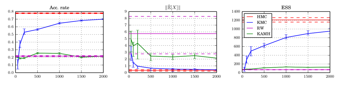
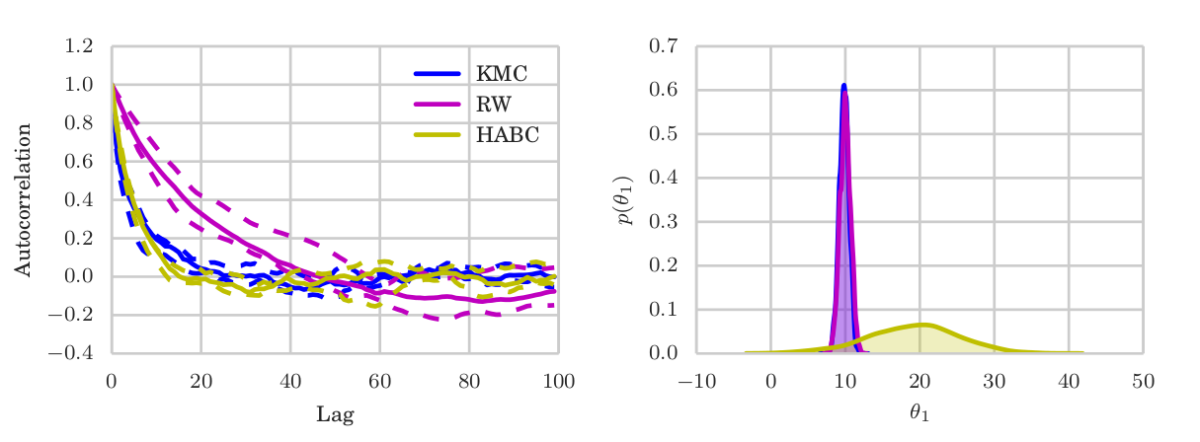
We argue that there exists a class of posterior distributions for that HMC is not available, while the distribution itself is still highly non-linear. You get them as easy as attempting binary classification with a Gaussian Process. Machine Learning doesn’t get more applied. Well, a bit: we sample the posterior distribution over the hyper-parameters using Pseudo-Marginal MCMC. The latter makes both likelihood and gradient intractable and the former in many cases has an interesting shape. See this plot which is the posterior of parameters of an Automatic Relevance Determination Kernel on the UCI Glass dataset. This is not an exotic problem at all, but it has all the properties we are after: non-linearity and higher order information unavailable. We cannot do HMC, so we are left with a random walk, which doesn’t work nicely here due to the non-linear shape.

The idea of our algorithm is to do a random walk in an infinite dimensional space. At least almost.

  • We run some method to get a rough sketch of the distribution we are after.
  • We then embed these points into a RKHS; some infinite dimensional mean and covariance operators are going on here, but I will spare you the details here.
  • In the RKHS, the chain samples are Gaussian, which corresponds to a manifold in the input space, which in some sense aligns with what we have seen of the target density yet.
  • We draw a sample $f$ from that Gaussian – random walk in the RKHS
  • This sample is in an infinite dimensional space, we need to map it back to the original space, just like in Kernel PCA
  • It turns out that is hard (nice word for impossible). So let’s just take a gradient step along some cost function that minimises distances in the way we want: \[\argmin_{x\in\mathcal{X}}\left\Vert k\left(\cdot,x\right)-f\right\Vert _{\mathcal{H}}^{2}\]
  • Cool thing: This happens in input space and gives us a point whose embedding is in some sense close to the RKHS sample.
  • Wait, everything is Gaussian! Let’s be mathy and integrate the RKHS sample (and the gradient step) out.

Et voilà, we get a Gaussian proposal distribution in input space\[q_{\mathbf{z}}(\cdot|x_{t})=\mathcal{N}(x_{t},\gamma^{2}I+\nu^{2}M_{\mathbf{z},x_{t}}HM_{\mathbf{z},x_{t}}^{\top}),\]where $\Mz=2\eta\left[\nabla_{x}k(x,z_{1})|_{x=y},\ldots,\nabla_{x}k(x,z_{n})|_{x=y}\right]$ is based on kernel gradients (which are all easy to get). This proposal aligns with the target density. It is clear (to me) that using this for sampling is better than just an isotropic one. Here are some pictures of bananas and flowers.

The paper puts this idea in the form of an adaptive MCMC algorithm, which learns the manifold structure on the fly. One needs to be careful about certain details, but that’s all in the paper. Compared to existing linear adaptive samplers, which adapt to the global covariance structure of the target, our version adapts to the local covariance structure. This can all also be mathematically formalised. For example, for the Gaussian kernel, the above proposal covariance becomes \[\left[\text{cov}[q_{\mathbf{z}(\cdot|y)}]\right]_{ij} = \gamma^{2}\delta_{ij} + \frac{4\nu^{2}}{\sigma^{4}}\sum_{a=1}^{n}\left[k(y,z_{a})\right]^{2}(z_{a,i}-y_{i})(z_{a,j}-y_{j}) +\mathcal{O}(n^{-1}),\] where the previous points $z_a$ influence the covariance, weighted by their similarity $k(y,z_a)$ to current point $y$.

Pretty cool! We also have a few “we beat all competing methods” plots, but I find those retarded and will spare them here – though they are needed for publication 😉

Dino and me have also written a pretty Python implementation (link) of the above, where the GP Pseudo Marginal sampling is done with Shogun’s ability to importance sample marginal likelihoods of non-conjugate GP models (link). Pretty cool!