$\DeclareMathOperator*{\argmin}{arg\,min}$ $\def\Mz{M_{\mathbf{z},y}}$

In this year’s ICML in Bejing, Arthur Gretton, presented our paper on Kernel Adaptive Metropolis Hastings [link, poster]. His talk slides are based on Dino Sejdinovic ones [link]. Pitty that I did not have travel funding. The Kameleon is furious!

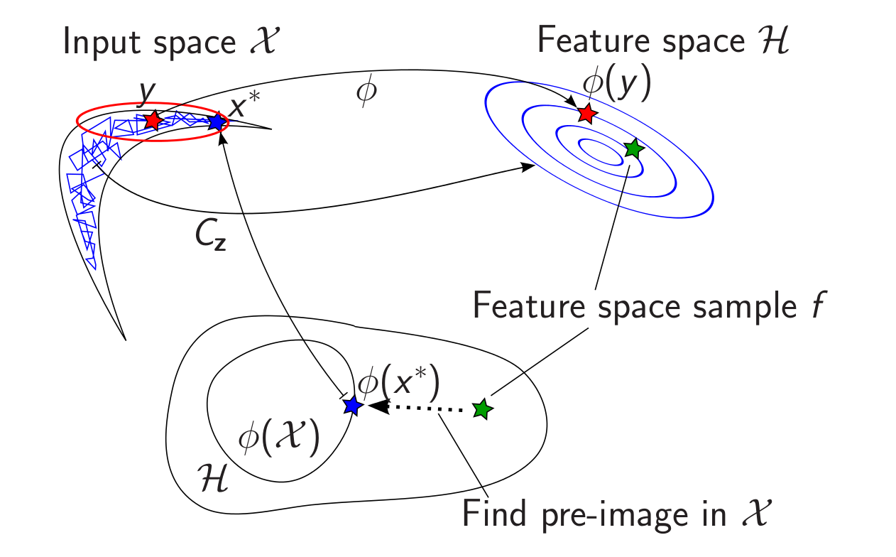
The idea of the paper is quite neat: It is basically doing Kernel-PCA to adapt a random walk Metropolis-Hastings sampler’s proposal based on the Markov chain’s history. Or, more fancy: Performing a random walk on an empirically learned non-linear manifold induced by an empirical Gaussian measure in a Reproducing Kernel Hilbert Space (RKHS). Sounds scary, but it’s not: the proposal distribution ends up being a Gaussian aligned to the history of the Markov chain.

We consider the problem of sampling from an intractable highly-nonlinear posterior distribution using MCMC. In such cases, the thing to do ™ usually is Hamiltonian Monte Carlo (HMC) (with all its super fancy extensions on Riemannian manifolds etc). The latter really is the only way to sample from complicated densities by using the geometry of the underlying space. However, in order to do so, one needs access to target likelihood and gradient.

We argue that there exists a class of posterior distributions for that HMC is not available, while the distribution itself is still highly non-linear. You get them as easy as attempting binary classification with a Gaussian Process. Machine Learning doesn’t get more applied. Well, a bit: we sample the posterior distribution over the hyper-parameters using Pseudo-Marginal MCMC. The latter makes both likelihood and gradient intractable and the former in many cases has an interesting shape. See this plot which is the posterior of parameters of an Automatic Relevance Determination Kernel on the UCI Glass dataset. This is not an exotic problem at all, but it has all the properties we are after: non-linearity and higher order information unavailable. We cannot do HMC, so we are left with a random walk, which doesn’t work nicely here due to the non-linear shape.

The idea of our algorithm is to do a random walk in an infinite dimensional space. At least almost.

• We run some method to get a rough sketch of the distribution we are after.
• We then embed these points into a RKHS; some infinite dimensional mean and covariance operators are going on here, but I will spare you the details here.
• In the RKHS, the chain samples are Gaussian, which corresponds to a manifold in the input space, which in some sense aligns with what we have seen of the target density yet.
• We draw a sample $f$ from that Gaussian – random walk in the RKHS
• This sample is in an infinite dimensional space, we need to map it back to the original space, just like in Kernel PCA
• It turns out that is hard (nice word for impossible). So let’s just take a gradient step along some cost function that minimises distances in the way we want: \[\argmin_{x\in\mathcal{X}}\left\Vert k\left(\cdot,x\right)-f\right\Vert _{\mathcal{H}}^{2}\]
• Cool thing: This happens in input space and gives us a point whose embedding is in some sense close to the RKHS sample.
• Wait, everything is Gaussian! Let’s be mathy and integrate the RKHS sample (and the gradient step) out.

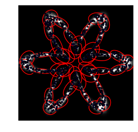
Et voilà, we get a Gaussian proposal distribution in input space\[q_{\mathbf{z}}(\cdot|x_{t})=\mathcal{N}(x_{t},\gamma^{2}I+\nu^{2}M_{\mathbf{z},x_{t}}HM_{\mathbf{z},x_{t}}^{\top}),\]where $\Mz=2\eta\left[\nabla_{x}k(x,z_{1})|_{x=y},\ldots,\nabla_{x}k(x,z_{n})|_{x=y}\right]$ is based on kernel gradients (which are all easy to get). This proposal aligns with the target density. It is clear (to me) that using this for sampling is better than just an isotropic one. Here are some pictures of bananas and flowers.

The paper puts this idea in the form of an adaptive MCMC algorithm, which learns the manifold structure on the fly. One needs to be careful about certain details, but that’s all in the paper. Compared to existing linear adaptive samplers, which adapt to the global covariance structure of the target, our version adapts to the local covariance structure. This can all also be mathematically formalised. For example, for the Gaussian kernel, the above proposal covariance becomes \[\left[\text{cov}[q_{\mathbf{z}(\cdot|y)}]\right]_{ij} = \gamma^{2}\delta_{ij} + \frac{4\nu^{2}}{\sigma^{4}}\sum_{a=1}^{n}\left[k(y,z_{a})\right]^{2}(z_{a,i}-y_{i})(z_{a,j}-y_{j}) +\mathcal{O}(n^{-1}),\] where the previous points $z_a$ influence the covariance, weighted by their similarity $k(y,z_a)$ to current point $y$.

Pretty cool! We also have a few “we beat all competing methods” plots, but I find those retarded and will spare them here – though they are needed for publication 😉

Dino and me have also written a pretty Python implementation (link) of the above, where the GP Pseudo Marginal sampling is done with Shogun’s ability to importance sample marginal likelihoods of non-conjugate GP models (link). Pretty cool!