More score matching for estimating gradients using the infinite dimensional kernel exponential family (e.g. for gradient-free HMC)! This paper tackles one of the most limiting practical characteristics of using the kernel infinite dimensional exponential family model in practice: the smoothness assumptions that come with the standard “swiss-army-knife” Gaussian kernel. These smoothness assumptions are blessing and curse at the same time: they allow for strong statistical guarantees, yet they can quite drastically restrict the expressiveness of the model.
To see this, consider a log-density model of the form (the “lite” estimator from our HMC paper) $$\log p(x) = \sum_{i=1}^n\alpha_ik(x,z_i)$$for “inducing points” $z_i$ (the points that “span” the model, could be e.g. the input data) and the Gaussian kernel $$k(x,y)=\exp\left(-\Vert x-y\Vert^2/\sigma\right)$$Intuitively, this means that the log-density is simply a set of layered Gaussian bumps — (infinitely) smooth, with equal degrees of variation everywhere. As the paper puts it
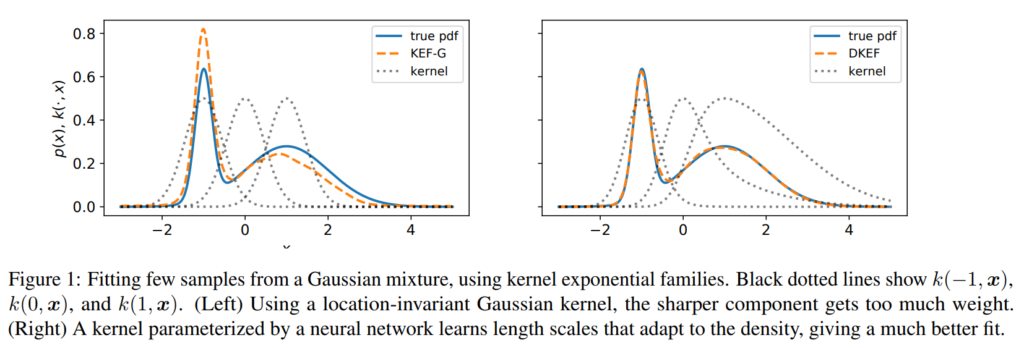
These kernels are typically spatially invariant, corresponding to a uniform smoothness assumption across the domain. Although such kernels are sufficient for consistency in the infinite-sample limit, the induced models can fail in practice on finite datasets, especially if the data takes differently-scaled shapes in different parts of the space. Figure 1 (left) illustrates this problem when fitting a simple mixture of Gaussians. Here there are two “correct” bandwidths, one for the broad mode and one for the narrow mode. A translation-invariant kernel must pick a single one, e.g. an average between the two, and any choice will yield a poor fit on at least part of the density
How can we learn a kernel that locally adapts to the density? Deep neural networks! We construct a non-stationary (i.e. location dependent) kernel using a deep network $\phi(x)$ on top a Gaussian kernel, i.e. $$k(x,y) = \exp\left(-\Vert \phi(x)-\phi(y)\Vert^2 / \sigma\right)$$ The network $\phi(x)$ is fully connected with softplus nonlinearity, i.e. $$\log(1+e^x)$$Softplus gives us some nice properties such as well-defined loss functions and a normalizable density model (See Proposition 2 in the paper for details).
However, we need to learn the parameters of the network. While kernel methods typically have nice closed-form solution with guarantees (and so does the original kernel exponential family model, see my post). Optimizing the parameters of ϕ(x)ϕ(x)ϕ(x) obviously makes things way more complicated: Whereas we could use a simple grid-search or black-box optimizer for a single kernel parameter, this approach here fails due to the number of parameters in ϕ(x)ϕ(x)12∫p0(x)∥∇xlogp(x)−∇xlogp0(x)∥2dx.
Could we use naive gradient descent? Doing so on our score-matching objective12∫p0(x)∥∇xlogp(x)−∇xlogp0(x)∥2dxwith logp(x)=∑ni=1αik(zi,x) and k(x,y)=exp(−∥x−y∥2/σ) will always overfit to the training data as the score (gradient error loss) can be made arbitrarily good by moving zi towards a data point and making σ go to zero. Stochastic gradient descent (the swiss-army-knife of deep learning) on the score matching objective might help, but would indeed produce very unstable updates.
Instead, we employed a two-stage training procedure that is conceptually motivated by cross-validation: we first do a closed-form update for the kernel model coefficients αiαiαi on one half of the dataset, then we perform a gradient step on the parameters of the deep kernel on the other half. We make use of auto-diff — extremely helpful here as we need to propagate gradients through a quadratic-form-style score matching loss, the closed-form kernel solution, and the network. This seems to work quite well in practice (the usual deep trickery to make it work applies). Take away: By using a two-stage procedure, where each gradient step involves a closed form (linear solve) solutions for the kernel coefficients αiαi we can fit this model reliably. See Algorithm 1 in the paper for more nitty-gritty details.
A cool extension of the paper would be to get rid of the sub-sampling/partitioning of the data and instead auto-diff through the leave-one-out error, which is closed form for these type of kernel models, see e.g. Wittawat’s blog post.
We experimentally compared the deep kernel exponential family to a number of other approaches based on likelihoods, normalizing flows, etc, and the results are quite positive, see the paper!
Naturally, as I have worked on using these gradients in HMC where the exact gradients are not available, I am very interested to see whether and how useful such a more expressive density model is. The case that comes to mind (and in fact motivated one of the experiments in the this paper) is the Funnel distribution (e.g. Neal 2003, picture by Stan), e.g.$$p(y,x) = \mathsf{normal}(y|0,3) * \prod_{n=1}^9 \mathsf{normal}(x_n|0,\exp(y/2)).$$
The mighty Funnel
This density historically was used as a benchmark for MCMC algorithms. Among others, HMC with second order gradients (Girolami 2011) perform much better due to their ability to adapt their step-sizes to the local scaling of the density — something that our new deep kernel exponential family is able to model. So I wonder: are there cases where such funnel-like densities arise in the context of say ABC or otherwise intractable gradient models? For those cases, an adaptive HMC sampler with the deep network kernel could improve things quite a bit.
We published a neat paper where we use the MMD as a critic for GANs. This contains a long overdue realisation of an asymptotic expression for the test power of the quadratic time MMD that we originally developed during my MSc thesis (looong time ago). [link]
We propose a method to optimize the representation and distinguishability of samples from two probability distributions, by maximizing the estimated power of a statistical test based on the maximum mean discrepancy (MMD). This optimized MMD is applied to the setting of unsupervised learning by generative adversarial networks (GAN), in which a model attempts to generate realistic samples, and a discriminator attempts to tell these apart from data samples. In this context, the MMD may be used in two roles: first, as a discriminator, either directly on the samples, or on features of the samples. Second, the MMD can be used to evaluate the performance of a generative model, by testing the model’s samples against a reference data set. In the latter role, the optimized MMD is particularly helpful, as it gives an interpretable indication of how the model and data distributions differ, even in cases where individual model samples are not easily distinguished either by eye or by classifier.
New paper online: Score matching goes Nystrom. With guarantees!
We propose a fast method with statistical guarantees for learning an exponential family density model where the natural parameter is in a reproducing kernel Hilbert space, and may be infinite dimensional. The model is learned by fitting the derivative of the log density, the score, thus avoiding the need to compute a normalization constant. We improved the computational efficiency of an earlier solution with a low-rank, Nystr\”om-like solution. The new solution retains the consistency and convergence rates of the full-rank solution (exactly in Fisher distance, and nearly in other distances), with guarantees on the degree of cost and storage reduction. We evaluate the method in experiments on density estimation and in the construction of an adaptive Hamiltonian Monte Carlo sampler. Compared to an existing score learning approach using a denoising autoencoder, our estimator is empirically more data-efficient when estimating the score, runs faster, and has fewer parameters (which can be tuned in a principled and interpretable way), in addition to providing statistical guarantees.
We propose Kamiltonian Kernel Hamiltonian Monte Carlo (KMC), a gradient-free adaptive MCMC algorithm based on Hamiltonian Monte Carlo (HMC). On target densities where classical HMC is not an option due to intractable gradients, KMC adaptively learns the target’s gradient structure by fitting an exponential family model in a Reproducing Kernel Hilbert Space. Computational costs are reduced by two novel efficient approximations to this gradient. While being asymptotically exact, KMC mimics HMC in terms of sampling efficiency, and offers substantial mixing improvements over state-of-the-art gradient free samplers. We support our claims with experimental studies on both toy and real-world applications, including Approximate Bayesian Computation and exact-approximate MCMC.
Motivation: HMC with intractable gradients.
Many recent applications of MCMC focus on models where the target density function is intractable. A very simple example is the context of Pseudo-Marginal MCMC (PM-MCMC), for example in Maurizio’spaper on Bayesian Gaussian Processes classification. In such (simple) models the marginal likelihood $p(\mathbf{y}|\theta )$ is unavailable in closed form, but only can be estimated. Performing Metropolis-Hastings style MCMC on $\hat{p}(\theta |\mathbf{y})$ results in a Markov chain that (remarkably) converges to the true posterior. So far so good. But no gradients.
Sometimes, people argue that for simple objects as latent Gaussian models, it is possible to side-step the intractable gradients by running an MCMC chain on the joint space $(\mathbf{f},\theta)$ of latent variables and hyper-parameters, which makes gradients available (and also comes with a set of other problems such as high correlations between $\mathbf{f}$ and $\theta$, etc). While I don’t want to get into this here (we doubt existence of a one-fits-all solution), there is yet another case where gradients are unavailable.
Approximate Bayesian Computation is based on the context where the likelihood itself is a black-box, i.e. it can only be simulated from. Imagine a physicist coming to you with three decades of intuition in the form of some Fortran code, which contains bits implemented by people who are not alive anymore — and he wants to do Bayesian inference on the code-parameters via MCMC… Here we have to give up on getting the exact answer, but rather simulate from a biased posterior. And of course, no gradients, no joint distribution.
Kamiltonian Monte Carlo starts as a Random Walk Metropolis (RWM) and then smoothly transitions into HMC. It explores the target at least as fast as RWM (we proof that), but improves the mixing in areas where it has been before.
We do this by learning the target gradient structure from the MCMC trajectory in an adaptive MCMC framework — using kernels. Every MCMC iteration, we update our gradient estimator with a decaying probability $a_t$ that ensures that we never stop updating, but update less and less, i.e. $$\sum_{t=1}^\infty \frac{1}{a_t}=\infty\qquad\text{and}\qquad\sum_{t=1} ^\infty \frac{1}{a_t^2}=0.$$ Christian Robert challenged our approach: using non-parametric density estimates for MCMC proposals directly is a bad idea: if certain parts of the space are not explored before adaptation effectively stopped, the sampler will almost never move there. For KMC (and for KAMH too) however, this is not a problem: rather than using density estimators as proposal directly, we use them for proposal construction. This way, these algorithms inherit ergodicity properties from random walks. I coded an example-demo here.
Kernel exponential families as gradient surrogates.
The density (gradient) estimator itself is an infinite dimensional exponential family model. More precisely, we model the un-normalised target log-density $\pi$ as an RKHS function $f\in\mathcal{H}$, i.e. $$\text{const}\times\pi(x)\approx\exp\left(\langle f,k(x,\cdot)\rangle_{{\cal H}}-A(f)\right),$$ which in particular implies $\nabla f\approx\nabla\log\pi.$ Surprisingly, and despite a complicated normaliser $A(f)$, such a model can be consistently fitted by directly minimising the expected $L^2$ distance of model and true gradient, $$J(f)=\frac{1}{2}\int\pi(x)\left\Vert \nabla f(x)-\nabla\log \pi (x)\right\Vert _{2}^{2}dx.$$ The magic word here is score-matching. You could ask: “Why not use kernel density estimation?” The answer: “Because it breaks in more than a few dimensions.” In contrast, we are actually able to make the above gradient estimator work in ~100 dimensions on Laptops.
Two approximations.
The über-cool infinite exponential family estimator, like all kernel methods, doesn’t scale nicely in the number $n$ of data used for estimation — and here neither in the in input space dimension $d$. Matrix inversion with costs $\mathcal{O}(t^3d^3)$ becomes a blocker, in particular as $t$ here is the growing number of MCMC iterations. KMC comes in two variants, which correspond to different approximations to the original kernel exponential family model.
KMC lite expresses the log-density in a smaller dimensional (yet growing) sub-space, via collapsing all $d$ input space dimensions into one. It takes the dual form $$f(x)=\sum_{i=1}^{n}\alpha_{i}k(x_{i},x),$$ where the $x_i$ are $n$ random sub-samples (just like KAMH) from the Markov chain history. Downside: KMC lite has to be re-estimated whenever the $x_i$ change. Advantage: The estimator’s tails vanish outside the $x_i$, i.e. $\lim_{\|x\|_{2}\to\infty}\|\nabla f(x)\|_{2}=0$, which translates into a geometric ergodicity result as we will see later.
KMC finite approximates the model as a finite dimensional exponential family in primal form, $$f(x)=\langle\theta,\phi_{x}\rangle_{{\cal H}_{m}}=\theta^{\top}\phi_{x},$$ where $x\in\mathbb{R}^{d}$ is embedded into a finite dimensional feature space $\phi_{x}\in{\cal H}_{m}=\mathbb{R}^{m}.$ While other choices are possible, we use the Randon Kitchen Sink framework: a $m$-dimensional data independent random Fourier basis. Advantage: KMC lite is an efficient on-line estimator that can be updated at constant costs in $t$ — we can fit it on all of the MCMC trajectory. Disadvantage: Its do not decay and our proof for geometric ergodicity of KMC lite does not apply.
Increasing dimensions.
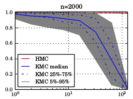
So far, we did not work out how the approximation errors propagate through the kernel exponential family estimator, but we plan to do that at some point. The paper contains an empirical study which shows that the gradients are good enough for HMC up to ~100 dimensions — Under a “Gaussian like smoothness” assumption. The below plots show the acceptance probability along KMC trajectories and quantify how “close” KMC proposals are to HMC proposals.
As a function in number of points $n$ and dimension $d$.
For a fixed number of points $n=2000$, as a function of dimension $d$.
For a fixed dimension $d=16$, as a function of number of points $n$.
How many points are needed to reach an acceptance rate of $0.1,…,0.7$, as a function of dimension $d$?
From RWM to HMC.
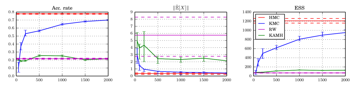
Using the well known and (ab)used Banana density as a target, we feed a non-adaptive version of KMC and friends with an increasing number of so-called “oracle” samples (iid from the target), and then quantify how well they mix. While this scenario is totally straw-man, it allows to compare the mixing behaviour of the algorithms after a long burn-in. The below plots show KMC transitioning from a random walk into something close to HMC as the number of “oracle” samples (x-axis) increases.ABC — Reduced simulations and no additional bias.
While there is another example in the paper, I want to show the ABC one here, which I find most interesting. Recall in ABC, the likelihood is not available. People often use synthetic likelihoods that are for example Gaussian, which induces an additional bias (in addition to ABC itself) but might improve statistical efficiency. In an algorithm called Hamiltonian ABC, such a synthetic likelihood is combined with stochastic gradient HMC (SG-HMC) via randomized finite differences, called simultaneous perturbation stochastic approximation (SPSA), which works as follows. To evaluate the gradient at a position $\theta$ in sampling space:
Generate a random SPSA mask $\Delta$ (set of binary directions) and compute the perturbed $\theta+\Delta$ and $\theta+\Delta$.
Interpolate linearly between them the perturbations. That is simulate from the ABC likelihood at both points, construct the synthetic likelihood, and use their difference.
The gradient is a (step-size dependent!) approximation to the unknown gradient of the (biased) synthetic likelihood model.
Perform a single stochastic HMC leapfrog step (adding friction as described in the SG-HMC paper)
Iterate for $L$ leapfrog iterations.
What I find slightly irritating is that this algorithm needs to simulate from the ABC likelihood in every leapfrog iteration — and then discards the gained information after a leapfrog step has been taken. How many leapfrog steps are common in HMC? Radford Neal suggests to start with $L\in[100,1000]$. Quite a few ABC simulations come with this! But there are more issues:
SG-HMC mixing. I found that stochastic gradient HMC mixes very poorly when the gradient noise large. Reducing noise costs even more ABC simulations. Wrongly estimated noise (non-stationary !?!) induces bias due to the “always accept” mentality. Step-size decreasing to account for that further hurts mixing.
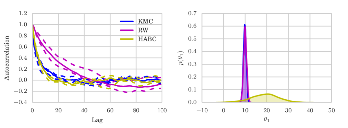
Bias. The synthetic likelihood can fail spectacularly, if the true likelihood is skewed for example.
KMC does not suffer from either of those problems: It keeps on improving its mixing as it sees more samples, while only requiring a single ABC simulation at each MCMC iterations — rather than HABC’s $2L$ (times noise-reduction-repetitions). It targets the true (modulo ABC bias) posterior, while accumulating information of the target (and its gradients) in the form of the MCMC trajectory.
But how do you choose the kernel parameter?
Often, this question is a threat for any kernel-based algorithm. For example, for the KAMH algorithm, it is completely unclear (to us!) how select these parameters in a principled way. For KMC, however, we can simply use cross-validation on the score matching objective function above. In practice, we use a black box optimisation procedure (for example CMA or Bayesian optimisation) to on-line update the kernel hyper-parameters every few MCMC iterations. See an example where our Python code does this here. Just like the updates to the gradient estimator itself, this can be done with a decaying probability to ensure asymptotic correctness.
In this year’s ICML in Bejing, Arthur Gretton, presented our paper on Kernel Adaptive Metropolis Hastings [link, poster]. His talk slides are based on Dino Sejdinovic ones [link]. Pitty that I did not have travel funding. The Kameleon is furious!
The idea of the paper is quite neat: It is basically doing Kernel-PCA to adapt a random walk Metropolis-Hastings sampler’s proposal based on the Markov chain’s history. Or, more fancy: Performing a random walk on an empirically learned non-linear manifoldinduced by an empirical Gaussian measure in aReproducing Kernel Hilbert Space (RKHS). Sounds scary, but it’s not: the proposal distribution ends up being a Gaussian aligned to the history of the Markov chain.
We consider the problem of sampling from an intractable highly-nonlinear posterior distribution using MCMC. In such cases, the thing to do ™ usually is Hamiltonian Monte Carlo (HMC) (with all its super fancy extensions on Riemannian manifolds etc). The latter really is the only way to sample from complicated densities by using the geometry of the underlying space. However, in order to do so, one needs access to target likelihood and gradient.
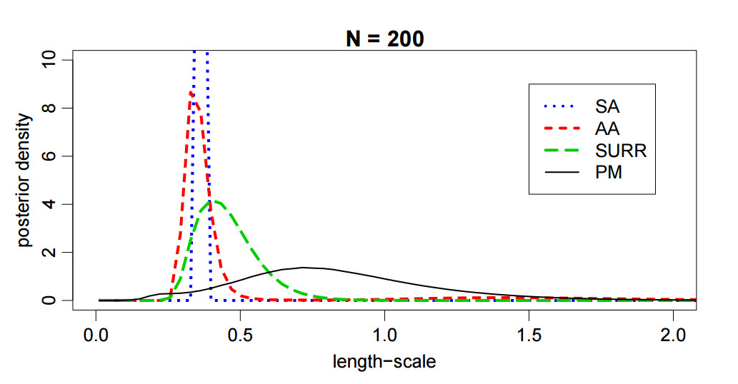
We argue that there exists a class of posterior distributions for that HMC is not available, while the distribution itself is still highly non-linear. You get them as easy as attempting binary classification with a Gaussian Process. Machine Learning doesn’t get more applied. Well, a bit: we sample the posterior distribution over the hyper-parameters using Pseudo-Marginal MCMC. The latter makes both likelihood and gradient intractable and the former in many cases has an interesting shape. See this plot which is the posterior of parameters of an Automatic Relevance Determination Kernel on the UCI Glass dataset. This is not an exotic problem at all, but it has all the properties we are after: non-linearity and higher order information unavailable. We cannot do HMC, so we are left with a random walk, which doesn’t work nicely here due to the non-linear shape.
The idea of our algorithm is to do a random walk in an infinite dimensional space. At least almost.
We run some method to get a rough sketch of the distribution we are after.
We then embed these points into a RKHS; some infinite dimensional mean and covariance operators are going on here, but I will spare you the details here.
In the RKHS, the chain samples are Gaussian, which corresponds to a manifold in the input space, which in some sense aligns with what we have seen of the target density yet.
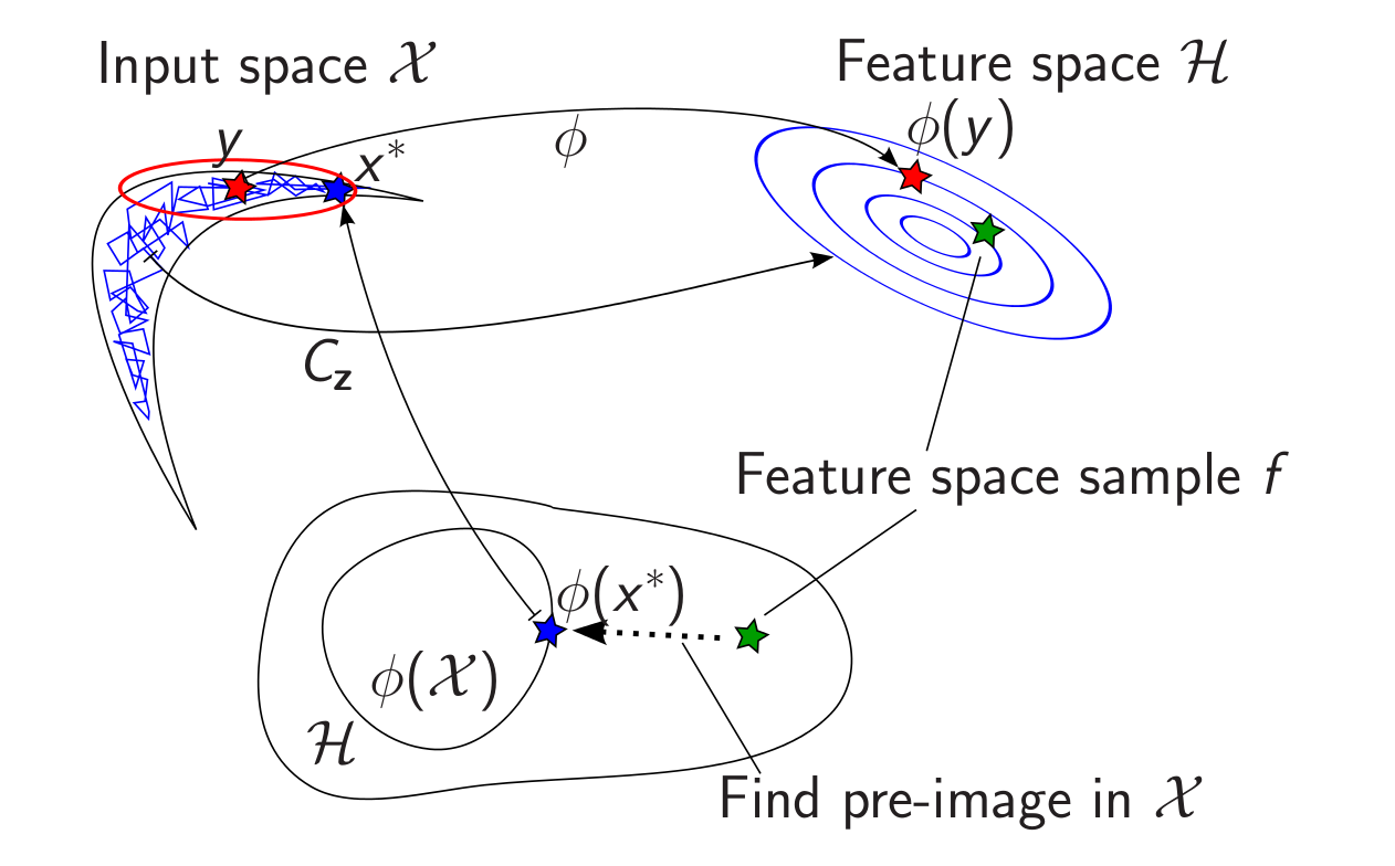
We draw a sample $f$ from that Gaussian – random walk in the RKHS
This sample is in an infinite dimensional space, we need to map it back to the original space, just like in Kernel PCA
It turns out that is hard (nice word for impossible). So let’s just take a gradient step along some cost function that minimises distances in the way we want: \[\argmin_{x\in\mathcal{X}}\left\Vert k\left(\cdot,x\right)-f\right\Vert _{\mathcal{H}}^{2}\]
Cool thing: This happens in input space and gives us a point whose embedding is in some sense close to the RKHS sample.
Wait, everything is Gaussian! Let’s be mathy and integrate the RKHS sample (and the gradient step) out.
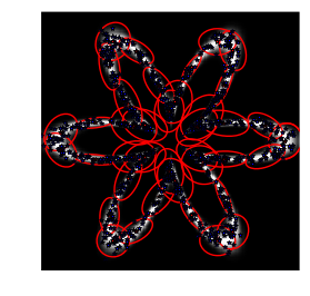
Et voilà, we get a Gaussian proposal distribution in input space\[q_{\mathbf{z}}(\cdot|x_{t})=\mathcal{N}(x_{t},\gamma^{2}I+\nu^{2}M_{\mathbf{z},x_{t}}HM_{\mathbf{z},x_{t}}^{\top}),\]where $\Mz=2\eta\left[\nabla_{x}k(x,z_{1})|_{x=y},\ldots,\nabla_{x}k(x,z_{n})|_{x=y}\right]$ is based on kernel gradients (which are all easy to get). This proposal aligns with the target density. It is clear (to me) that using this for sampling is better than just an isotropic one. Here are some pictures of bananas and flowers.
The paper puts this idea in the form of an adaptive MCMC algorithm, which learns the manifold structure on the fly. One needs to be careful about certain details, but that’s all in the paper. Compared to existing linear adaptive samplers, which adapt to the global covariance structure of the target, our version adapts to the local covariance structure. This can all also be mathematically formalised. For example, for the Gaussian kernel, the above proposal covariance becomes \[\left[\text{cov}[q_{\mathbf{z}(\cdot|y)}]\right]_{ij} = \gamma^{2}\delta_{ij} + \frac{4\nu^{2}}{\sigma^{4}}\sum_{a=1}^{n}\left[k(y,z_{a})\right]^{2}(z_{a,i}-y_{i})(z_{a,j}-y_{j}) +\mathcal{O}(n^{-1}),\] where the previous points $z_a$ influence the covariance, weighted by their similarity $k(y,z_a)$ to current point $y$.
Pretty cool! We also have a few “we beat all competing methods” plots, but I find those retarded and will spare them here – though they are needed for publication 😉
Dino and me have also written a pretty Python implementation (link) of the above, where the GP Pseudo Marginal sampling is done with Shogun’s ability to importance sample marginal likelihoods of non-conjugate GP models (link). Pretty cool!
NIPS 2012 is already over. Unfortunately, I could not go due to the lack of travel funding. However, as mentioned a few weeks ago, I participated in one paper which is closely related to my Master’s project with Arthur Gretton and Massi Pontil. Optimal kernel choice for large-scale two-sample tests. We recently set up a page for the paper where you can download my Matlab implementation of the paper’s methods. Feel free to play around with that. I am currently finishing implementing most methods into the SHOGUN toolbox. We also have a poster which was presented at NIPS. See below for all links. Update: I have completed the kernel selection framework for SHOGUN, it will be included in the next release. See the base class interface here. See an example to use it: single kernel (link) and combined kernels (link). All methods that are mentioned in the paper are included. I also updated the shogun tutorial (link).
At its core, the paper describes a method for selecting the best kernel for two-sample testing with the linear time MMD. Given a kernel $k$ and terms
$$h_k((x_{i},y_{i}),((x_{j},y_{j}))=k(x_{i},x_{i})+k(y_{i},y_{i})-k(x_{i},y_{j})-k(x_{j},y_{i}),$$
the linear time MMD is their empirical mean,
$$\hat\eta_k=\frac{1}{m}\sum_{i=1}^{m}h((x_{2i-1},y_{2i-1}),(x_{2i},y_{2i})),$$
which is a linear time estimate for the squared distance of the mean embeddings of the distributions where the $x_i, y_i$ come from. The quantity allows to perform a two-sample test, i.e. to tell whether the underlying distributions are different.
Given a finite family of kernels $\mathcal{K}$, we select the optimal kernel via maximising the ratio of the MMD statistic by a linear time estimate of the standard deviation of the terms
$$k_*=\arg \sup_{k\in\mathcal{K}}\frac{ \hat\eta_k}{\hat \sigma_k},$$
where $\hat\sigma_k^2$ is a linear time estimate of the variance $\sigma_k^2=\mathbb{E}[h_k^2] – (\mathbb{E}[h_k])^2$ which can also be computed in linear time and constant space. We give a linear time and constant space empirical estimate of this ratio. We establish consistency of this empirical estimate as
$$ \left\vert \sup_{k\in\mathcal{K}}\hat\eta_k \hat\sigma_k^{-1} -\sup_{k\in\mathcal{K}}\eta_k\sigma_k^{-1}\right\vert=O_P(m^{-\frac{1}{3}}).$$
In addition, we describe a MKL style generalisation to selecting weights of convex combinations of a finite number of baseline kernels,
$$\mathcal{K}:={k : k=\sum_{u=1}^d\beta_uk_u,\sum_{u=1}^d\beta_u\leq D,\beta_u\geq 0, \forall u\in{1,…,d}},$$
via solving the quadratic program
$$\min_\beta { \beta^T\hat{Q}\beta : \beta^T \hat{\eta}=1, \beta\succeq 0},$$
where $\hat{Q}$ is the positive definite empirical covariance matrix of the $h$ terms of all pairs of kernels.
We then describe three experiments to illustrate
That our criterion outperforms existing methods on synthetic and real-life datasets which correspond to hard two-sample problems
Why multiple kernels can be an advantage in two-sample testing
See also the description of my Master’s project (link) for details on the experiments.
I wrote my Bachelor thesis in 2009/2010 in Duisburg, supervised by Prof. Hoffmann, Bioinformatics, Essen, and Prof. Pauli, Intelligent systems, Duisburg.
The work is about classification of amino acid sequences using SVM and string kernels. In particular, I compared the Distant Segments kernel by Sébastian Boisvert to a standard Spectrum kernel on a HIV dataset. In addition, I described a bisection based method to search for the soft-margin parameter of the underlying SVM, which outperformed a standard grid-search.


 We argue that there exists a class of posterior distributions for that HMC is not available, while the distribution itself is still highly non-linear. You get them as easy as attempting binary classification with a