Together with Louis Ellam, Iain Murray, and Mark Girolami, we just published / arXived a new article on dealing with large Gaussian models. This is slightly related to the open problem around the GMRF model in our Russian Roulette paper back a while ago.
We propose a determinant-free approach for simulation-based Bayesian inference in high-dimensional Gaussian models. We introduce auxiliary variables with covariance equal to the inverse covariance of the model. The joint probability of the auxiliary model can be computed without evaluating determinants, which are often hard to compute in high dimensions. We develop a Markov chain Monte Carlo sampling scheme for the auxiliary model that requires no more than the application of inverse-matrix-square-roots and the solution of linear systems. These operations can be performed at large scales with rational approximations. We provide an empirical study on both synthetic and real-world data for sparse Gaussian processes and for large-scale Gaussian Markov random fields.
Article is here. Unfortunately, the journal is not open-access, but the arXiv version is.
New paper online: Score matching goes Nystrom. With guarantees!
We propose a fast method with statistical guarantees for learning an exponential family density model where the natural parameter is in a reproducing kernel Hilbert space, and may be infinite dimensional. The model is learned by fitting the derivative of the log density, the score, thus avoiding the need to compute a normalization constant. We improved the computational efficiency of an earlier solution with a low-rank, Nystr\”om-like solution. The new solution retains the consistency and convergence rates of the full-rank solution (exactly in Fisher distance, and nearly in other distances), with guarantees on the degree of cost and storage reduction. We evaluate the method in experiments on density estimation and in the construction of an adaptive Hamiltonian Monte Carlo sampler. Compared to an existing score learning approach using a denoising autoencoder, our estimator is empirically more data-efficient when estimating the score, runs faster, and has fewer parameters (which can be tuned in a principled and interpretable way), in addition to providing statistical guarantees.
This project is yet another method to scale up Bayesian inference via sub-sampling. But unlike most other work on this field, we do not use sub-sampling within an MCMC algorithm to simulate from the posterior distribution of interest. Rather, we use sub-sampling to create a series of easier inference problems, whose results we then combine to get the answer to the question we were originally asking — in an estimation sense, without full posterior simulation. I’ll describe the high-level ideas now.
Updates on the project:
Jun: I was invited to present the work at the Big Bayes workshop in Oxford.
Feb: We got featured in Xi’an’s Og, including a nice discussion in the comments
Feb: I presented the work at the Oxford Machine Learning lunch. Good discussion with the crowd. We will probably change the name to Big Bayes without sub-sampling bias.
Bounded variance (even for growing $N$) and can be controlled.
No sub-sampling bias is introduced. The method inherits the usual finite time bias from MCMC though.
Not limited to certain models or inference schemes.
Trade off redundancy in the data against computational savings.
Perform competitive in practice.
Bayesian inference usually involves integrating a functional $\varphi:\Theta\rightarrow\mathbb{R}$ over a posterior distribution $$\phi=\int d\theta\varphi(\theta)\underbrace{p(\theta|{\cal D})}_{\text{posterior}},$$ where $$p(\theta|{\cal D})\propto\underbrace{p({\cal D}|\theta)}_{\text{likelihood data}}\underbrace{p(\theta)}_{\text{prior}}.$$ For example, to compute the predictive posterior mean for a linear regression model. This is often done by constructing an MCMC algorithm to simulate $m$ approximately iid samples from approximately $\theta^{(j)}\sim p(\theta|{\cal D})$ (the second “approximately” here refers to the fact that MCMC is biased for any finite length of the chain, and the same is true for our method) and then performing Monte Carlo integration $$\phi\approx\frac{1}{m}\sum_{j=1}^{m}\varphi(\theta^{(j)}).$$ Constructing such Markov chains can quickly become infeasible as usually, all data needs to be touched in every iteration. Take for example the standard Metropolis-Hastings transition kernel to simulate from $\pi(\theta)\propto p(\theta|{\cal D})$, where at a current point $\theta^{(j)}$, a proposed new point $\theta’\sim q(\theta|\theta^{(j)})$ is accepted with probability $$\min\left(\frac{\pi(\theta’)}{\pi(\theta^{(j)})}\times\frac{q(\theta^{(j)}|\theta’)}{q(\theta’|\theta^{(j)})},1\right).$$ Evaluating $\pi$ requires to iterate through the whole dataset. A natural question therefore is: is it possible to only use subsets of $\mathcal{D}$?
Existing work. There has been a number of papers that tried to use sub-sampling within the transition kernel of MCMC:
An adaptive sub-sampling approach: Use concentration bounds to decide whether to accept/reject. Quantify error, establish convergence.
Firefly Monte Carlo: Augment the state space of the Markov chain and combine with a lower bound on the likelihood
All these methods have in common that they either introduce bias (in addition to the bias caused by MCMC), have no convergence guarantees, or mix badly. This comes from the fact that it is extremely difficult to modify the Markov transition kernel and maintain its asymptotic correctness.
In our paper, we therefore take a different perspective. If the goal is to solve an estimation problem as the one above, we should not make our life hard trying to simulate. We construct a method that directly estimates posterior expectations — without simulating from the full posterior, and without introducing sub-sampling bias.
The idea is very simple:
Construct a series of partial posterior distributions $\tilde{\pi}_{l}:=p({\theta|\cal D}_{l})\propto p({\cal D}_{l}|\theta)p(\theta)$ from subsets of sizes $$\vert\mathcal{D}_1\vert=a,\vert\mathcal{D}_2\vert=2^{1}a,\vert\mathcal{D}_3\vert=2^{2}a,\dots,\vert\mathcal{D}_L\vert=2^{L-1}a$$ of the data. This gives $$p(\theta)=\tilde{\pi}_{0}\rightarrow\tilde{\pi}_{1}\rightarrow\tilde{\pi}_{2}\rightarrow\dots\rightarrow\tilde{\pi}_{L}=\pi_{N}=p({\theta|\cal D}).$$
Compute posterior expectations $\phi_{t}:=\hat{\mathbb{E}}_{\tilde{\pi}_{t}}\{\varphi(\theta)\}$ for each of the partial posteriors. This can be done for example MCMC, or other inference methods. This gives a sequence of real valued partial posterior expectations — that converges to the true posterior.
Use the debiasing framework, by Glynn & Rhee. This is a way to unbiasedly estimate the limit of a sequence without evaluating all elements. Instead, one randomly truncates the sequence at term $T$ (which should be “early” in some sense, $T$ is a random variable), and then computes $$\phi^*=\sum_{t=1}^T \frac{\phi_{t}-\phi_{t-1}}{\mathbb{P}\left[T\geq t\right]}.$$ This is now an unbiased estimator for the full posterior expectation. The intuition is that one can rewrite any sequence limit as a telescopic sum $$\lim_{t\to\infty} \phi_t=\sum_{t=1}^\infty (\phi_{t}-\phi_{t-1})$$ and then randomly truncate the infinite sum and divide through truncation probabilities to leave the expectation untouched, i.e. $$\mathbb{E}[\phi^*]=\phi,$$where $\phi$ is the sequence limit.
In the paper, we choose the random truncation time as $$\mathbb{P}(T=t)\propto 2^{-\alpha t}.$$ From here, given a certain choice of $\alpha$, it is straight-forward to show the average computational cost of this estimator is $\mathcal{O} (N^{1-\alpha}),$ which is sub-linear in $N$. We also show that variance is finite and can be bounded even when $N\to\infty$. This statement is modulo certain conditions on the $\phi_t$. In addition, the choice of the $\alpha$-parameter of the random truncation time $T$ is crucial for performance. See the paper for details how to set it.
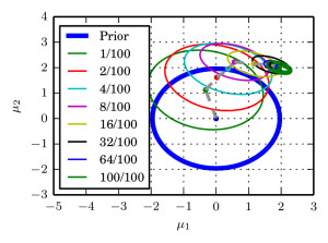
Conentration Gaussian
Debiasing illustration
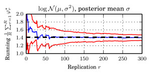
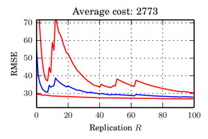
Experimental results are very encouraging. On certain models, we are able to estimate model parameters accurately before plain MCMC even has finished a single iteration. Take for example a log-normal model $$p(\mu,\sigma|{\cal D})\propto\prod_{i=1}^{N}\log{\cal N}(x_{i}|\mu,\sigma^{2})\times\text{flat prior}$$ and functional $$\varphi((\mu,\sigma))=\sigma.$$ We chose the true parameter $\sigma=\sqrt{2}$ and ran our method in $N=2^{26}$ data. The pictures below contain some more details.
Debiasing
Used data in debiasing
Convergence of statistic
Comparison to stochastic variational inference is something we only thought of quite late in the project. As we state in the paper, as mentioned in my talks, and as pointed out in feedback from the community, we cannot do uniformly better than MCMC. Therefore, comparing to full MCMC is tricky — even though there exist trade-offs of data redundancy and model complexity that we can exploit as showed in the above example. Comparing to other “limited data” schemes really showcases the strength (and generality) of our method.
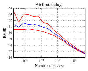
We chose to compare against “Gaussian Processes for Big Data“, which puts together a decade of engineering of variational lower bounds, the inducing features framework for GPs, and stochastic variational inference to solve Gaussian Process regression on roughly a million data points. In contrast, our scheme is very general and not specifically designed for GPs. However, we are able to perform similar to this state of the art method. On predicting airtime delays, we reach a slightly lower RMSE at comparable computing effort. The paper contains details on our GP, which is slightly different (but comparable) to the one used in the GP for Big Data paper. Another neat detail of the GP example is that the likelihood does not factorise, which is in contrast to most other Bayesian sub-sampling schemes.
Debiasing
Convergence of RMSE
GP for Big Data
In summary, we arrive at
Computational costs sub-linear in $N$
No introduced sub-sampling bias (in addition to MCMC, if used)
Finite, and controllable variance
A general scheme that is not limited to MCMC nor to factorising likelihoods
A scheme that trades off redundancy for computational savings
A practical scheme that performs competitive to state-of-the-art methods and that has no problems with transition kernel design.
See the paper for a list of weaknesses and open problems.
Last week, I went to the i-like workshop at Oxford university. Pretty cool! All of Britain’s statisticians were there and I met many of them for the first time. Check out my two posters (Russian Roulette, Kernel Adaptive Metropolis Hastings). Talks were amazing – as in last NIPS, the main trend is on estimating likelihoods (well, that’s the name of the program), either using some other random process such as importance sampling a latent model’s marginal likelihood (aka Pseudo-Marginal MCMC), or directly sub-sampling likelihoods or gradients.
These things are important in Machine Learning too, and it is very nice to see the field growing together (even-though there was a talk by a Statistician spending lots of time on re-inventing belief propagation and Junction tree ideas – always such a pitty if this happens simply because communities do not talk to each other enough). Three talks that I really found interesting:
Remi Bardenet talked about sub-sampling approaches to speed up MCMC. This is quite related to the Austerity in MCMC land paper by Welling & Co, with the difference that his tests do not suffer from small number of points in the hypothesis test to decide accept/reject.
Chris Sherlock talked about optimal rates and scaling for Pseudo-Marginal MCMC. There finally are some nice heuristics how to scale PM estimates in a way that the number of iid samples per computation time is optimal. Interestingly, the acceptance rate and the variance of the likelihood estimate can be tweaked separately.
Jim Griffin gave a very interesting talk on adaptive MCMC on discrete, in particular binary, state-spaces – he used them for feature selection (in ML language). His algorithm automatically learns global mutations rates for each of the positions. However, it doesn’t take any correlations between the features into account. This might be a very interesting application for our fancy Kameleon sampler (arxiv, code), thinking about this!
Finally, I presented two posters, the one on Playing Russian Roulette with Intractable Likelihoods that I already presented in Reykjavik, and (with Dino) a new poster (link) on the Kernel Adaptive Metropolis Hastings Kameleon that I mentioned above. The corresponding paper is hopefully published very soon. Talking to other scientists about my own work is just great!