An ICML 2019 paper, together with Kevin Li, Dougal Sutherland, and Arthur Gretton. Code by Kevin.
More score matching for estimating gradients using the infinite dimensional kernel exponential family (e.g. for gradient-free HMC)! This paper tackles one of the most limiting practical characteristics of using the kernel infinite dimensional exponential family model in practice: the smoothness assumptions that come with the standard “swiss-army-knife” Gaussian kernel. These smoothness assumptions are blessing and curse at the same time: they allow for strong statistical guarantees, yet they can quite drastically restrict the expressiveness of the model.
To see this, consider a log-density model of the form (the “lite” estimator from our HMC paper) $$\log p(x) = \sum_{i=1}^n\alpha_ik(x,z_i)$$for “inducing points” $z_i$ (the points that “span” the model, could be e.g. the input data) and the Gaussian kernel $$k(x,y)=\exp\left(-\Vert x-y\Vert^2/\sigma\right)$$Intuitively, this means that the log-density is simply a set of layered Gaussian bumps — (infinitely) smooth, with equal degrees of variation everywhere. As the paper puts it
These kernels are typically spatially invariant, corresponding to a uniform smoothness assumption across the domain. Although such kernels are sufficient for consistency in the infinite-sample limit, the
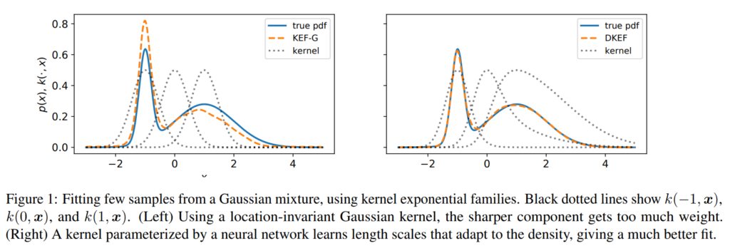
induced models can fail in practice on finite datasets, especially if the data takes differently-scaled shapes in different parts of the space. Figure 1 (left) illustrates this problem when fitting a simple mixture of Gaussians. Here there are two “correct” bandwidths, one for the broad mode and one for the narrow mode. A translation-invariant kernel must pick a single one, e.g. an average between the two, and any choice will yield a poor fit on at least part of the density

How can we learn a kernel that locally adapts to the density? Deep neural networks! We construct a non-stationary (i.e. location dependent) kernel using a deep network $\phi(x)$ on top a Gaussian kernel, i.e. $$k(x,y) = \exp\left(-\Vert \phi(x)-\phi(y)\Vert^2 / \sigma\right)$$ The network $\phi(x)$ is fully connected with softplus nonlinearity, i.e. $$\log(1+e^x)$$Softplus gives us some nice properties such as well-defined loss functions and a normalizable density model (See Proposition 2 in the paper for details).
However, we need to learn the parameters of the network. While kernel methods typically have nice closed-form solution with guarantees (and so does the original kernel exponential family model, see my post). Optimizing the parameters of ϕ(x) obviously makes things way more complicated: Whereas we could use a simple grid-search or black-box optimizer for a single kernel parameter, this approach here fails due to the number of parameters in 12∫p0(x)∥∇xlogp(x)−∇xlogp0(x)∥2dx.
Could we use naive gradient descent? Doing so on our score-matching objectivewith and will always overfit to the training data as the score (gradient error loss) can be made arbitrarily good by moving towards a data point and making go to zero. Stochastic gradient descent (the swiss-army-knife of deep learning) on the score matching objective might help, but would indeed produce very unstable updates.
Instead, we employed a two-stage training procedure that is conceptually motivated by cross-validation: we first do a closed-form update for the kernel model coefficients αi on one half of the dataset, then we perform a gradient step on the parameters of the deep kernel on the other half. We make use of auto-diff — extremely helpful here as we need to propagate gradients through a quadratic-form-style score matching loss, the closed-form kernel solution, and the network. This seems to work quite well in practice (the usual deep trickery to make it work applies). Take away: By using a two-stage procedure, where each gradient step involves a closed form (linear solve) solutions for the kernel coefficients we can fit this model reliably. See Algorithm 1 in the paper for more nitty-gritty details.
A cool extension of the paper would be to get rid of the sub-sampling/partitioning of the data and instead auto-diff through the leave-one-out error, which is closed form for these type of kernel models, see e.g. Wittawat’s blog post.
We experimentally compared the deep kernel exponential family to a number of other approaches based on likelihoods, normalizing flows, etc, and the results are quite positive, see the paper!
Naturally, as I have worked on using these gradients in HMC where the exact gradients are not available, I am very interested to see whether and how useful such a more expressive density model is. The case that comes to mind (and in fact motivated one of the experiments in the this paper) is the Funnel distribution (e.g. Neal 2003, picture by Stan), e.g.$$p(y,x) = \mathsf{normal}(y|0,3) * \prod_{n=1}^9 \mathsf{normal}(x_n|0,\exp(y/2)).$$

This density historically was used as a benchmark for MCMC algorithms. Among others, HMC with second order gradients (Girolami 2011) perform much better due to their ability to adapt their step-sizes to the local scaling of the density — something that our new deep kernel exponential family is able to model. So I wonder: are there cases where such funnel-like densities arise in the context of say ABC or otherwise intractable gradient models? For those cases, an adaptive HMC sampler with the deep network kernel could improve things quite a bit.
