Step by step, my project enters a final state 🙂
Last week, I added new data generation methods, which are used from a new example for independence tests with HSIC. It demonstrates that the HSIC based test is able to capture dependence which is induced by rotating data that has zero correlation — one of the problems from the paper [1]. Here is a picture; the question is: are the two dimensions dependent? Or moreover, is a test able to capture that? (correlation is almost zero, dependence is induced via rotation)

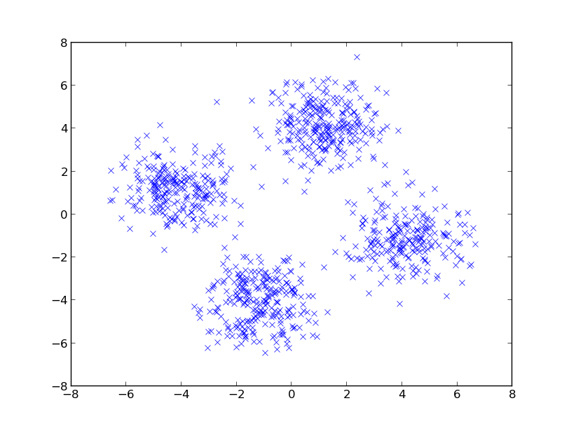
I also realised that my current class structure had problems doing bootstrapping for HSIC, so I re-factored a bit. Bootstrapping is now also available for HISC using the same code that does it for two-sample-tests. I also removed some redundancy — both independence and two-sample tests are very similar problems and implementations should share code where possible.

Another thing that was missing so far is to compute test thresholds; so far, only p-values could be computed. Since different people have different tastes about this, I added both methods. Checking a test statistic against a threshold is straight-forward and gives a binary answer; computing a p-value gives the position of the test statistic in the null-distribution — this contains more information. To compute thresholds, one needs the inverse CDF function for the null-distribution. In the bootstrapping case, it is easy since simply the sample that corresponds to a certain quantile has to be reported. For cases where a normal- or gamma-distribution was fitted, I imported some more routines from the nice ALGLIB toolbox.

For this week, I plan to continue with finishing touches, documentation, examples/tests, etc. Another idea I had is to make the linear time MMD test work with SHOGUN’s streaming features, since the infinite or streaming data case is the main area for its usage.

[1]: Gretton, A., Fukumizu, K., Teo, C., & Song, L. (2008). A kernel statistical test of independence. Advances in Neural Information Processing Systems

I spend quite some fraction of last week on something which is not really related my project: trying to make cross-validation possible for multi-class MKL (multiple kernel learning) machines using my framework from last year’s GSoC. To this end, I added subset support to SHOGUN’s combined features class; and then went for a bunch of bugs that prevented it from working. But it now does! So cross-validation should now be possible within a lot more situations. Thanks to Eric who reported all the problems.

Apart from that, I worked on documentation for the new statistical testing framework. I added doxygen class descriptions, see for example CQuadraticTimeMMD. More important, I started writing a section for the SHOGUN tutorial, a book-like description of all algorithms. We hope that it will grow in the future. You can find the \(\LaTeX\) sources at github. We should/will add a live pdf download soon.

Another minor thing I implemented is a data generator class. I think it is nice to illustrate new algorithms with data that is not fixed (aka load a file). The nice thing about this is that it is available for examples from all interfaces — so far I implemented this separately for c++ and python; this is more elegant now. I bet some of the others projects will need similar methods for their demos too; so please extend the class!

This week, I will add more data generation methods to the generator, in particular data that can be used to illustrate the recently implemented HSIC test for independence. Reference datasets are quite complicated, so this might take a while. Another thing we recently changed is a new framework for unit-tests, so I will write these for all new methods I created recently.

Last week was a mixed one. Next to new examples, tests, bugfixes, and helper methods, the biggest implementation is an automatic kernel selection algorithm for the linear time MMD. This is one thing that I worked on during my Master project at UCL.
It selects optimal optimal kernel weights for kernel of the family
\[
\mathcal{K}:=\{k : k=\sum_{u=1}^d\beta_uk_u,\sum_{u=1}^d\beta_u\leq D,\beta_u\geq0, \forall u\in\{1,…,d\}\}
\]
by solving the convex program
\[
\min \{ \beta^T\hat{Q}\beta : \beta^T \hat{\eta}=1, \beta\succeq0\}
\]
where \(\hat{Q}\) is a linear time estimate of the covariance of the MMD estimates and \(\hat{\eta}\) is a linear time estimate of the MMD.

I already described this a few weeks ago, when the method was developed. It is now integrated into SHOGUN. Efficient kernel selection, yeah 🙂 It uses a convex solver called libqp, which is by Vojtech Franc, one of the mentors of this year’s GSoC. Still, I need to think of a nice way of embedding it into SHOGUN’s model selection framework, which isn’t as straight-forward as it first seems.

This week, bug-hunting continues with a bug that gives wrong results during cross-validation on multi-class machines. Afterwards, I will try to polish my code so far a bit, especially documentation (and tutorial); and continue on more examples/demo for the new framework for statistical testing.

Finally, I started on kernel based (in)dependence tests last week. These are tests that try to find out whether for two random variables \(\textbf{x},\textbf{y} \) are independent, i.e. whether their joint distribution factorises into the individual ones. The null hypothesis (that may be rejected) is \[ H_0:P_\textbf{x}P_\textbf{y}=P_{\textbf{x}\textbf{y}}\]

These kind of tests basically work like two-sample tests: Given one set of samples from each random variable
\[ Z=(X,Y)=\{(x_1,y_1,…,(x_m,y_m)\}\]
a test statistic is computed and then compared against the distribution of the statistic under the null-hypothesis. If the position is in an upper part of it, the null-hypothesis is rejected since it is unlikely that the current value was generated by it.

The class of independence tests I will implement for my project are all based on the Hilbert Schmidt independence criterion (HSIC), which takes out the above procedure to an reproducing kernel Hilbert space (RKHS). The (biased version of the) HSIC statistic itself is simply given by
\[\text{HSIC}_b(Z)=\frac{1}{m^2}\text{trace}(KHLH)\]
where \(K,L \) are kernel matrices of the input samples \( X,Y\) in some RKHS and \(H=I-\frac{1}{m}\textbf{1}\textbf{1}^T\) is a centring matrix.

I integrated a general modular framework for independence tests into SHOGUN. The HSIC class is the first kernel-independence test that works. Interfaces are very similar to the two-sample test, however, they are not quite the same for various reasons. That’s why there is another class for independence testing next to the one for two-sample testing.

As for the two-sample tests, the null-distribution may simply be approximated by bootstrapping, i.e. merging the samples and computing the statistic for many times. This is now possible for any independence test. Another method to approximate the null-distribution for HSIC is fitting a Gamma distribution [1] as

\[m\text{HSIC}=\frac{x^{\alpha-1}\exp(-\frac{x}{\beta})}{\beta^\alpha \Gamma(\alpha)} \] where
\[\alpha=\frac{(\textbf{E}(\text{HSIC}_b(Z)))^2}{\text{var}(\text{HSIC}_b(Z))} \quad \text{and}\quad\beta=\frac{m\text{var}(\text{HSIC}_b(Z))}{\textbf{E}(\text{HSIC}_b(Z))}\]

It’s also already implemented! There are already modular interfaces for the new classes and some simple tests. I will extend these during this weak. Time passes fast: The mid-term-evaluation is this week already. I pretty much enjoyed the first half 🙂

[1]: Gretton, A., Fukumizu, K., Teo, C., & Song, L. (2008). A kernel statistical test of independence.

Last week’s changes were all rather subtle:

• I created some first modular examples in python,
• fixed this big bug in the model selection trees I talked about last week (nasty!),
• added some convenience methods for the two-sample-test constructors (there is now a new method in CFeatures to append feature objects)
• and corrected a bunch of bugs on the fly.

This week, I will do some more work on the examples and then start working on independence testing.

Last week, I have been working silently (no Internet connection) on finishing all MMD related tests. What is new is a distinction between biased/unbiased test statistics for the quadratic MMD, and the Gaussian approximation of the null-distribution for the linear time MMD – and more tests.

Since the linear time MMD, defined as
\[\text{MMD}_l^2=\frac{1}{m}\sum_{i=1}^{m}h((x_{2i-1},y_{2i-1}),(x_{2i},y_{2i}))\]
where
\[h((x_{i},y_{i}),((x_{j},y_{j}))=k(x_{i},x_{i})+k(y_{i},y_{i})-k(x_{i},y_{j})-k(x_{j},y_{i})\]
is normally distributed both in null- and alternative distribution, one can easily compute test-threshold and p-values using the variance of the h-values of the above term as a proxy for the real variance (The null-distribution has zero mean). For large sample sizes, this is an accurate and very cheap way to perform the test: The statistic has to be computed only once whereas bootstrapping would need a few hundred iterations. Another reason why the linear time MMD is well suited for large scale problems.

I also started on integrating my code into the modular interfaces of SHOGUN and will produce some first python examples next week.

Jacob (Gaussian Process Regression project), who uses and extends parts of my model selection code from last years GSoC has found a serious problem in SHOGUN’s parameter trees for model selection. I hope to fix it this week – complicated.

When all mentioned things are done, I might start with dependence testing next week.

Since all threshold methods that I implemented so far are quite unintuitive and hard to verify, I spent last week writing tests for most of their parts. I created test-cases based on fixed and random datasets (mainly taken from the papers where the methods were introduced), in which results are compared against MATLAB implementations of the same problem. For most cases, the difference is asserted to be smaller than 10E-15.

Although it takes a lot of time and effort, I believe these automatic tests should come with every more complicated method in SHOGUN. I remember quite some cases where I spent an hour on finding an error that would have been easily caught by a test.

I hope to finish all all statistical tests based on the quadratic MMD this week. I still need to implement the biased version (which can be used along with the threshold methods) and a possibility for choosing the type of statistic to use. I also plan to implement the linear time MMD and corresponding tests (Gaussian approximation of null-distribution). I won’t have Internet access this week since I am in nowhere in Poland — so expect a larger patch at the end of the week.

I finally finished my exams last week and can now work full-time for GSoC and my Master project. Puh! 🙂

Last week, I implemented two methods to compute a threshold for the quadratic time MMD test:

1. A test based on the Eigenspectrum of the kernel matrix of the joint samples. This is a nice and computationally efficient idea from [1]. The basic idea is that for the case \(P=Q\), the biased estimate of the null-distribution converges in distribution:
   \[ m\text{MMD}^2_b \rightarrow \sum_{l=1}^\infty \lambda_l z_l^2\]
   where \(z_l \sim \mathcal{N}(0,2)\) i.i.d. and  \(\lambda_l\) are Eigenvalues of which the empirical estimates \(\hat{\lambda}_l\) are given by the Eigenvalues of the centred kernel matrix \(\tilde{K}=HKH\) where \(K_{ij}=k(x_i,x_j)\). Its possible to sample the null-distribution using these estimates and to compute a p-value or threshold using the resulting samples.
2. A heuristic method, also from [1],  that approximates the null-distribution with a gamma-distribution where the first two moments are matched. I.e.
   \[m\text{MMD}_b(Z) \sim \frac{x^{\alpha-1}\exp(-\frac{x}{\beta})}{\beta^\alpha \Gamma(\alpha)}\] where \[ \alpha=\frac{(\textbf{E}(\text{MMD}_b(Z)))^2}{\text{var}(\text{MMD}_b(Z))}\quad \text{and}\quad \beta=\frac{m\text{var}(\text{MMD}_b(Z))}{(\textbf{E}(\text{MMD}_b(Z)))^2}\]

Both methods need some some distribution function (\(\Gamma\), etc), which I integrated from ALGLIB. I added some tests to ensure that results equal to these obtained with MATLAB. Along with that come some SGVector based wrappers for SHOGUN functions (sorting, eigenvalues, etc).

Next week, I will do some fine-tuning on the implemented methods and then create tests which illustrate all methods.

[1]: Gretton, A., Fukumizu, K., & Harchaoui, Z. (2011). A fast, consistent kernel two-sample test.

Last week, I was again very busy with exams and doing experiments for a NIPS submission.

The latter is somehow related to my GSoC project, and I will implement it once the other stuff is done:
We developed a method for selecting optimal coefficients of a non-negative combination of kernels for the linear time (=large scale) MMD-two-sample test. The criterion that is optimised for is the ratio of the linear MMD \(\eta_k\) by its standard deviation \(\sigma_k \), i.e.
\[ k_*=\arg \sup_{k\in\mathcal{K}} \eta_k \sigma_k^{-1}\]. That is equivalent to solving the quadratic program
\[
\min \{ \beta^T\hat{Q}\beta : \beta^T \hat{\eta}=1, \beta\succeq0\}
\]
where the combination of kernels is given by
\[
\mathcal{K}:=\{k : k=\sum_{u=1}^d\beta_uk_u,\sum_{u=1}^d\beta_u\leq D,\beta_u\geq0, \forall u\in\{1,…,d\}\}
\]
\(\hat{Q}\) is a linear time estimate of the covariance of the MMD estimates and \(\hat{\eta}\) is a linear time estimate of the MMD using the above kernel combinations.

Apart from that, I implemented a method to approximate the null-distribution of the quadratic time MMD, which is based on the Eigenspectrum of the kernel matrix of the merged samples from the two distributions, based on [1]. It still needs to be compared against the MATLAB implementation. It comes with some minor helper functions around matrix algebra.

This week, I will finally have my last exam and then continue on the advanced methods for computing test thresholds.

[1]: Gretton, A., Fukumizu, K., & Harchaoui, Z. (2011). A fast, consistent kernel two-sample test.

I am currently quite busy with my exams, however, the last three will be done soon and I still managed to do initial sketches for the statistical testing framework along with helping on solving problems that occurred because of the massive changes that are currently happening to SHOGUN’s label and multi-class system.

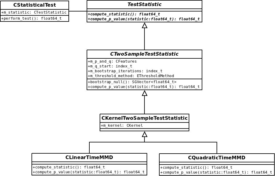
Here you can find an UML diagram of the class structure so far. I implemented first simple kernel-two-sample-tests — the ones based on the linear and the quadratic time MMD metric. For computing a p-value, these two may approximate their null-distribution using a (brute-force) bootstrapping approach based on shuffling data of the two underlying distributions and then computing the statistic multiple times. The bootstrapping code will work for any two-sample based test.

Next steps are: Advanced methods for estimating Null-distributions for the MMD tests.

I also worked with Arthur (mentor) on a version of the MMD that is related to my Master project: A convex combination of (arbritary) kernels for the linear time MMD where the optimal weights are learned by solving a quadratic program. I might implement that into SHOGUN as well. (Who can help me how to interface the QP-solver of SHOGUN?)